RL Circuits. Non-instantaneous current, time constant, and magnetic energy
The online RL circuit simulations on this page allow you to interactively explore how current and voltage evolve when an inductor is connected or disconnected through a resistor. Through the simulations, you can observe how the inductor initially opposes the flow of current, how the current grows following an exponential curve, and how, after a sufficient amount of time, it reaches the value imposed by the resistor in steady state. You can also measure the time constant 𝜏 = 𝐿/𝑅, compare the rates of rise and fall for different values of L and R, and intuitively understand how this parameter controls the entire circuit dynamics.
This Thematic Unit is part of our Circuits collection
What are RL circuits
An RL circuit is a connection made up of a resistor and an inductor which, when powered by a voltage source, displays dynamic behaviour: the current does not change instantaneously, but evolves gradually over time. Unlike purely resistive circuits—in which the current reaches its final value immediately—in an RL circuit, the presence of the inductor introduces a transient process governed by the creation or disappearance of a magnetic field. This dynamic causes the circuit to pass through three clearly differentiated stages: an initial instant in which the inductor opposes the change in current, a transient phase in which the current rises or falls following an exponential law, and a final state in which the inductor behaves as a simple conductor. RL circuits are essential for understanding how magnetic energy is stored and released, how time delays are generated, and how current variations are controlled in electronic and power applications.
Growth and decay of current in an RL circuit
In an RL circuit, the current does not change instantaneously when the power source is connected or disconnected. The inductor opposes any sudden variation and forces the current to evolve gradually, following an exponential law both in the process of increase and in the process of decrease. This delayed response is the fundamental characteristic of RL circuits and explains many of their practical uses.
Current growth
When a voltage is applied to an RL circuit, the current does not reach its final value immediately: the inductor opposes the change and makes the current rise progressively. During this transient process, part of the energy supplied by the source is stored in the magnetic field of the inductor, which explains the initial resistance to current flow and the exponential shape of the growth.
Current decay
When the power supply is interrupted, the current does not drop abruptly either: the inductor tries to maintain it and generates a voltage that forces its circulation until the stored magnetic energy dissipates. This process also follows an exponential law and is responsible for phenomena such as voltage spikes that appear when opening an inductive circuit. The time constant τ = R·C
The time constant τ = L/R
The evolution of current in an RL circuit is determined by the time constant τ, a quantity which sets the speed at which the circuit responds to changes. Just like in RC circuits, this constant defines the duration of the transient phase and allows us to predict how the current will rise or fall depending on the values of its components.
Physical meaning of τ
The time constant τ = L/R indicates the characteristic time it takes for the current to change appreciably. After an interval equal to τ, the current has covered about 63% of the distance between its initial value and its final value, which allows the speed of the transient process to be described precisely.
How L and R affect the speed of the process
A higher value inductor increases the time constant and makes the current change more slowly, while a larger resistor reduces it and speeds up the transition. The relationship between these two components determines whether the circuit responds quickly or slowly to any variation in applied voltage.
Exponential voltage and current curves
The temporal evolution of an RL circuit can be represented by exponential curves describing how current and voltage change during the processes of growth and decay. These graphs allow direct visualisation of the circuit’s transient phase and understanding of how the time constant sets the speed at which the steady state is reached.
Current growth curve
When the power source is connected, the current increases from zero following a rising exponential curve. The initial slope is at its maximum and decreases as the inductor completes the formation of its magnetic field, gradually approaching the final value set by the resistor.
Current decay curve
When the power source is disconnected, the current decreases following a falling exponential curve. The inductor releases the energy stored in its magnetic field, maintaining the current for a brief interval before it drops almost to zero.
Reading and interpreting the graphs
In both curves, the key point is the time constant τ, which marks the speed of the process: after a time equal to τ, the current has completed approximately 63% of the total change. These graphs allow clear identification of the transient phase, the steady state, and the influence of the values of L and R on the circuit’s response.
Series and parallel inductor connections
Inductors can be combined to obtain an equivalent inductance that simplifies circuit analysis. Just as with resistors and capacitors, these combinations allow adjustment of the circuit’s temporal response, as the total inductance directly influences the time constant τ = L/R. The combination rules are opposite to those for capacitors and reflect how magnetic effects are added or shared when several coils act together.
Inductors in series
When several inductors are connected in series, their inductances add directly , because the same current flow passes through all the coils and the magnetic fields are added:
Leq = L1 + L2 + L3 +…
A greater equivalent inductance makes the circuit respond more slowly to changes in current.
Inductors in parallel
In a parallel connection, the current can split between several paths, so the equivalent inductance decreases . The relationship is obtained by summing the reciprocals of each inductance:
1/Leq = 1/L1 + 1/L2 + 1/L3 + …
and, in the particular case of two inductors, it can be written as:
Leq = (L1 · L2) / (L1 + L2)
A smaller equivalent inductance speeds up the circuit’s response to any variation in applied voltage.
Practical applications of RL circuits
RL circuits are used in a wide variety of systems where it is necessary to control the temporal evolution of current, filter signals, or manage magnetic energy. Their ability to oppose abrupt changes in current makes them essential in low-pass and high-pass filters, where inductance determines which frequencies are attenuated or allowed through. They are also used to generate delays and smooth transients in switching stages, soft starts, and protection against current spikes. In power electronics, inductors store and release energy in a controlled manner, allowing regulation of voltages, limiting of currents, and improvement of efficiency in converters and switched power supplies. Thanks to these properties, RL circuits are key elements both in low-signal electronic applications and in larger-scale power systems.
Explore the exciting STEM world with our free, online, simulations and accompanying companion courses! With them you’ll be able to experience and learn hands-on. Take this opportunity to immerse yourself in virtual experiences while advancing your education – awaken your scientific curiosity and discover all that the STEM world has to offer!
RL circuit simulations
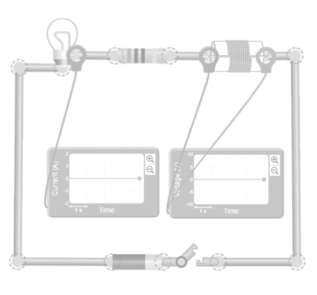
Simple RL circuit with current growth and decay
In this first simulation, we study the fundamental behavior of an RL circuit. To do this, just as on the RC page, we use the AC Circuit Construction Kit – Virtual Laboratory, which allows us to visualize in real time the evolution of the current and voltage in each circuit element.
The simulation consists of a DC battery, a light bulb, and an inductor connected in series, along with a switch that allows the user to start and stop the process of current rise and fall. The light bulb acts as a resistive element and as a visual indicator: its brightness is dim at the beginning, when the current is practically zero, and increases progressively as the inductor allows the current to stabilize.
In addition to this qualitative observation, the simulation includes an ammeter in series and a voltmeter connected to the inductor, allowing users to simultaneously view the voltage and current graphs as a function of time. In this way, the visitor can see that the current rises following an exponential curve that gradually approaches the final value set by the resistor, while the voltage across the inductor drops from a high initial value to practically zero. This time-domain representation makes it clear that the current in an RL circuit does not change instantaneously, but is governed by the time constant τ = L/R, which determines how quickly the system responds to a change. The experiment provides the conceptual foundation necessary to understand how more complex circuits behave and how the choice of resistance and inductance values determines the speed at which a circuit establishes or interrupts the current.
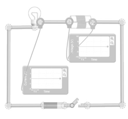
RL circuit with a variable resistor, exploring the time constant
This second simulation delves into the influence of the time constant on the evolution of the current in an RL circuit. To do this, a simple circuit is used consisting of a DC battery, a switch, an adjustable resistor, a light bulb, and an inductor connected in series. Additionally, a graphical ammeter is incorporated into the circuit—displaying the current in real time—and a graphical voltmeter connected across the coil terminals, allowing the voltage drop across the inductor to be viewed simultaneously throughout the process.
The simulation works very intuitively: simply change the resistance value to see how the speed at which the current stabilizes in the circuit changes. When the resistance is set to a high value, the final current is lower and the time constant decreases, so the rise curve becomes steeper and the bulb reaches its steady brightness in less time. Conversely, when the resistance is reduced, the final current increases and the time constant grows, causing the current to take longer to stabilize and the bulb to light up more slowly and gradually. These differences are clearly reflected in both the current graph and the inductor voltage, which shows higher values when the current changes rapidly and decreases smoothly as the system approaches steady state.
Giants of science
“If I have seen further, it is by standing on the shoulders of giants”
Isaac Newton
James Clerk Maxwell
–
Michael Faraday
–
Become a giant
Principles of Modeling, Simulations, and Control for Electric Energy Systems
Principles of Electric Circuits | 电路原理
Electrotechnique I
Electromagnetic Compatibility Essentials
Professional development for Educators
HP AI Teacher Academy
Learn Like a Pro: Science-Based Tools to Become Better at Anything
BlendedX: Blended Learning with edX
Support kids’ projects: Web development
Giants of science
“If I have seen further, it is by standing on the shoulders of giants”
Isaac Newton
James Clerk Maxwell
–
Michael Faraday
–
Become a giant
Principles of Modeling, Simulations, and Control for Electric Energy Systems
Principles of Electric Circuits | 电路原理
Electrotechnique I
Electromagnetic Compatibility Essentials
Professional development for Educators
Assessment Design with AI
Teaching with Physical Computing: Assessment of Project-Based Learning
Teaching and Learning in the Era of AI
Teach teens computing: Object-oriented Programming in Python
Test your knowledge
You may also be interested
Last simulations
To learn and experience
Take your knowledge to the next level with science kits and hands-on tools that connect theory with experimentation
Calculadora científica

Teachers essentials
Notion
Organize your notes, tasks, and projects in one place. Notion combines notes, lists, and calendars in one flexible space.
Canva
Design presentations, diagrams, and infographics with easy-to-use templates and professional results
Genially
Create interactive content, presentations, and educational games in a simple and visual way
Desmos
The most intuitive graphing calculator to explore mathematics and create dynamic classroom activities
Tinkercad
Design in 3D and simulate electronic circuits for free; it’s the perfect tool for simple robotics projects
Your Infinite Library
Enjoy the freedom to explore millions of titles and a curated selection of magazines on any device
Join Prime for students and young adults
The best series. Millions of songs. All included with your subscription.
Science made fun
Learn with the best courses
edX
Online courses from leading universities and companies. Learn practical skills and earn professional certifications
Coursera
Courses from leading universities and companies. Learn practical skills and earn professional certifications
Udemy
Thousands of online courses tailored to your level. Learn at your own pace with expert instructors

